Profiling

Capturing traces

When running Reactant, it is possible to capture traces using the XLA profiler. These traces can provide information about where the XLA specific parts of program spend time during compilation or execution. Note that tracing and compilation happen on the CPU even though the final execution is aimed to run on another device such as GPU or TPU. Therefore, including tracing and compilation in a trace will create annotations on the CPU.

Let's setup a simple function which we can then profile

using Reactant

x = Reactant.to_rarray(randn(Float32, 100, 2))
W = Reactant.to_rarray(randn(Float32, 10, 100))
b = Reactant.to_rarray(randn(Float32, 10))

linear(x, W, b) = (W * x) .+ b

linear (generic function with 1 method)

The profiler can be accessed using the Reactant.with_profiler function.

Reactant.with_profiler("./") do
    mylinear = Reactant.@compile linear(x, W, b)
    mylinear(x, W, b)
end

10×2 ConcretePJRTArray{Float32,2}:
   7.35441    1.76483
   4.50912    2.67234
 -10.1758     2.20272
  11.1799     9.02824
   6.69894  -14.8104
   4.57778   -6.69169
  -7.58647    7.38649
  -4.99009  -12.9242
   8.35313   -2.6326
  -7.42291   -4.03929

Running this function should create a folder called plugins in the folder provided to Reactant.with_profiler which will contain the trace files. The traces can then be visualized in different ways.

Note

For more insights about the current state of Reactant, it is possible to fetch device information about allocations using the Reactant.XLA.allocatorstats function.

Perfetto UI

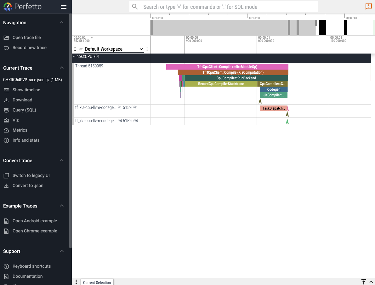
The first and easiest way to visualize a captured trace is to use the online perfetto.dev tool. Reactant.with_profiler has a keyword parameter called create_perfetto_link which will create a usable perfetto URL for the generated trace. The function will block execution until the URL has been clicked and the trace is visualized. The URL only works once.

Reactant.with_profiler("./"; create_perfetto_link=true) do
    mylinear = Reactant.@compile linear(x, W, b)
    mylinear(x, W, b)
end

Note

It is recommended to use the Chrome browser to open the perfetto URL.

Tensorboard

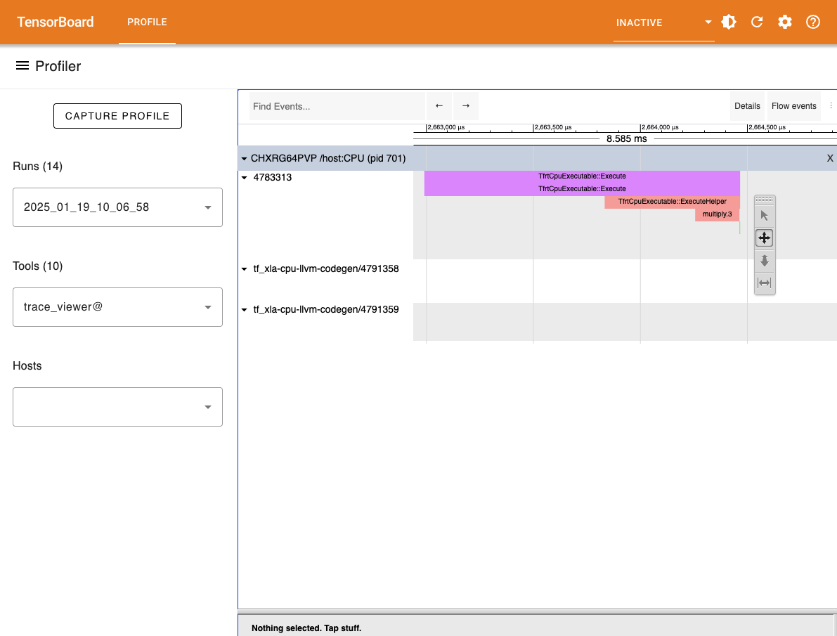
Another option to visualize the generated trace files is to use the tensorboard profiler plugin. The tensorboard viewer can offer more details than the timeline view such as visualization for compute graphs.

First install tensorboard and its profiler plugin:

pip install tensorboard tensorboard-plugin-profile

And then run the following in the folder where the plugins folder was generated:

tensorboard --logdir ./

Adding Custom Annotations

By default, the traces contain only information captured from within XLA. The Reactant.Profiler.annotate function can be used to annotate traces for Julia code evaluated during tracing.

Reactant.Profiler.annotate("my_annotation") do
    # Do things...
end

The added annotations will be captured in the traces and can be seen in the different viewers along with the default XLA annotations. When the profiler is not activated, then the custom annotations have no effect and can therefore always be activated.