Profiling
Quick profiling in your terminal
Note
This is only meant to be used for quick profiling or programmatically accessing the profiling results. For more detailed and GUI friendly profiling proceed to the next section.
Simply replace the use of Base.@time or Base.@timed with Reactant.Profiler.@time or Reactant.Profiler.@timed. We will automatically compile the function if it is not already a Reactant compiled function (with sync=true).
using Reactant

x = Reactant.to_rarray(randn(Float32, 100, 2))
W = Reactant.to_rarray(randn(Float32, 10, 100))
b = Reactant.to_rarray(randn(Float32, 10))

linear(x, W, b) = (W * x) .+ b

Reactant.@time linear(x, W, b)
┌ Debug: Profiling directory: /home/runner/.julia/scratchspaces/3c362404-f566-11ee-1572-e11a4b42c853/reactant_profiling/jl_QTp39C
└ @ Reactant.Profiler ~/work/Reactant.jl/Reactant.jl/src/Profiler.jl:626
WARNING: All log messages before absl::InitializeLog() is called are written to STDERR
I0000 00:00:1784141574.634857 4202 profiler_session.cc:121] Profiler session initializing.
I0000 00:00:1784141574.634927 4202 profiler_session.cc:136] Profiler session started.
I0000 00:00:1784141574.635253 4202 profiler_session.cc:84] Profiler session collecting data.
I0000 00:00:1784141574.635813 4202 save_profile.cc:239] Collecting XSpace to repository: /home/runner/.julia/scratchspaces/3c362404-f566-11ee-1572-e11a4b42c853/reactant_profiling/jl_QTp39C/plugins/profile/2026_07_15_18_52_54/runnervm5mmn9.xplane.pb
I0000 00:00:1784141574.636010 4202 save_profile.cc:212] Creating directory: /home/runner/.julia/scratchspaces/3c362404-f566-11ee-1572-e11a4b42c853/reactant_profiling/jl_QTp39C/plugins/profile/2026_07_15_18_52_54
I0000 00:00:1784141574.636132 4202 save_profile.cc:218] Dumped gzipped tool data for trace.json.gz to /home/runner/.julia/scratchspaces/3c362404-f566-11ee-1572-e11a4b42c853/reactant_profiling/jl_QTp39C/plugins/profile/2026_07_15_18_52_54/runnervm5mmn9.trace.json.gz
I0000 00:00:1784141574.636161 4202 profiler_session.cc:167] Profiler session tear down.
┌ Debug: Starting XProf gRPC server...
└ @ Reactant.Profiler ~/work/Reactant.jl/Reactant.jl/src/Profiler.jl:598
┌ Debug: Initializing XProf stubs for worker service at 0.0.0.0:41309
└ @ Reactant.Profiler ~/work/Reactant.jl/Reactant.jl/src/Profiler.jl:397
I0000 00:00:1784141574.650942 4202 stub_factory.cc:163] Created gRPC channel for address: 0.0.0.0:41309
┌ Debug: Starting XProf gRPC server on port 41309
└ @ Reactant.Profiler ~/work/Reactant.jl/Reactant.jl/src/Profiler.jl:413
I0000 00:00:1784141574.651316 4202 grpc_server.cc:94] Server listening on 0.0.0.0:41309 with max_concurrent_requests 1
I0000 00:00:1784141574.659736 4202 xplane_to_tools_data_with_profile_processor.cc:142] serving tool: memory_profile with options: {} using ProfileProcessor session_id: /home/runner/.julia/scratchspaces/3c362404-f566-11ee-1572-e11a4b42c853/reactant_profiling/jl_QTp39C/plugins/profile/2026_07_15_18_52_54
I0000 00:00:1784141574.659748 4202 xplane_to_tools_data_with_profile_processor.cc:165] Using local processing for tool: memory_profile
I0000 00:00:1784141574.659750 4202 memory_profile_processor.cc:47] Processing memory profile for host: runnervm5mmn9
I0000 00:00:1784141574.660047 4202 xplane_to_tools_data_with_profile_processor.cc:170] Total time for tool memory_profile: 304.323us session_id: /home/runner/.julia/scratchspaces/3c362404-f566-11ee-1572-e11a4b42c853/reactant_profiling/jl_QTp39C/plugins/profile/2026_07_15_18_52_54
I0000 00:00:1784141574.672965 4202 xplane_to_tools_data_with_profile_processor.cc:142] serving tool: op_profile with options: {} using ProfileProcessor session_id: /home/runner/.julia/scratchspaces/3c362404-f566-11ee-1572-e11a4b42c853/reactant_profiling/jl_QTp39C/plugins/profile/2026_07_15_18_52_54
I0000 00:00:1784141574.672981 4202 xplane_to_tools_data_with_profile_processor.cc:165] Using local processing for tool: op_profile
I0000 00:00:1784141574.672984 4202 multi_xplanes_to_op_stats.cc:118] ConvertMultiXSpaceToCombinedOpStatsWithCache: Started
I0000 00:00:1784141574.673030 4202 multi_xplanes_to_op_stats.cc:134] ConvertMultiXSpaceToCombinedOpStatsWithCache: Cache miss, calling ConvertMultiXSpacesToCombinedOpStats
I0000 00:00:1784141574.673032 4202 multi_xplanes_to_op_stats.cc:45] ConvertMultiXSpacesToCombinedOpStats: Started. Number of XSpaces: 1
I0000 00:00:1784141574.673036 4202 multi_xplanes_to_op_stats.cc:55] ConvertMultiXSpacesToCombinedOpStats: Starting to process XSpace 0/1
I0000 00:00:1784141574.673160 4202 derived_timeline.cc:693] GenerateDerivedTimeLines: creating derived_timeline_trace_events XprofThreadPoolExecutor
I0000 00:00:1784141574.673169 4202 xprof_thread_pool_executor.cc:22] Creating derived_timeline_trace_events XprofThreadPoolExecutor with 4 threads.
I0000 00:00:1784141574.673380 4202 derived_timeline.cc:705] GenerateDerivedTimeLines: waiting for derived_timeline_trace_events threads to join
I0000 00:00:1784141574.673699 4202 derived_timeline.cc:709] GenerateDerivedTimeLines: derived_timeline_trace_events threads joined successfully
I0000 00:00:1784141574.674037 4202 derived_timeline.cc:758] GenerateDerivedTimeLines: creating ProcessTensorCorePlanes XprofThreadPoolExecutor
I0000 00:00:1784141574.674050 4202 xprof_thread_pool_executor.cc:22] Creating ProcessTensorCorePlanes XprofThreadPoolExecutor with 4 threads.
I0000 00:00:1784141574.674197 4202 derived_timeline.cc:769] GenerateDerivedTimeLines: waiting for ProcessTensorCorePlanes threads to join
I0000 00:00:1784141574.674549 4202 derived_timeline.cc:772] GenerateDerivedTimeLines: ProcessTensorCorePlanes threads joined successfully
I0000 00:00:1784141574.677896 4202 xplane_to_op_stats.cc:405] ConvertXSpaceToOpStats: creating op_stats_threads XprofThreadPoolExecutor
I0000 00:00:1784141574.677918 4202 xprof_thread_pool_executor.cc:22] Creating op_stats_threads XprofThreadPoolExecutor with 4 threads.
I0000 00:00:1784141574.678076 4202 xplane_to_op_stats.cc:461] ConvertXSpaceToOpStats: Scheduled 0 OpMetricsDb generation tasks.
I0000 00:00:1784141574.678299 4202 xplane_to_op_stats.cc:417] ConvertXSpaceToOpStats: Combining 0 op_metrics_dbs.
I0000 00:00:1784141574.678306 4202 xplane_to_op_stats.cc:422] ConvertXSpaceToOpStats: Finished combining op_metrics_dbs.
I0000 00:00:1784141574.678513 4202 xplane_to_op_stats.cc:687] ConvertXSpaceToOpStats: Final OpStats size: 222 bytes (0.000211716 MiB).
I0000 00:00:1784141574.678581 4202 multi_xplanes_to_op_stats.cc:67] ConvertMultiXSpacesToCombinedOpStats: Finished processing XSpace 0.
I0000 00:00:1784141574.678596 4202 multi_xplanes_to_op_stats.cc:72] ConvertMultiXSpacesToCombinedOpStats: Finished extracting all 1 OpStats. Time: 5.566058ms
I0000 00:00:1784141574.678604 4202 multi_xplanes_to_op_stats.cc:85] ConvertMultiXSpacesToCombinedOpStats: Starting ComputeStepIntersectionToMergeOpStats.
I0000 00:00:1784141574.678606 4202 multi_xplanes_to_op_stats.cc:94] ConvertMultiXSpacesToCombinedOpStats: Finished ComputeStepIntersectionToMergeOpStats in 1.353us
I0000 00:00:1784141574.678609 4202 multi_xplanes_to_op_stats.cc:99] ConvertMultiXSpacesToCombinedOpStats: Starting CombineAllOpStats.
I0000 00:00:1784141574.678613 4202 multi_xplanes_to_op_stats.cc:106] ConvertMultiXSpacesToCombinedOpStats: Finished CombineAllOpStats in 3.176us
I0000 00:00:1784141574.678615 4202 multi_xplanes_to_op_stats.cc:109] ConvertMultiXSpacesToCombinedOpStats: Overall Finished in 5.58305ms
I0000 00:00:1784141574.678618 4202 multi_xplanes_to_op_stats.cc:138] ConvertMultiXSpaceToCombinedOpStatsWithCache: Starting to write cache file.
I0000 00:00:1784141574.678697 4202 multi_xplanes_to_op_stats.cc:145] ConvertMultiXSpaceToCombinedOpStatsWithCache: Finished writing cache file.
I0000 00:00:1784141574.678701 4202 multi_xplanes_to_op_stats.cc:149] ConvertMultiXSpaceToCombinedOpStatsWithCache: Overall Finished in 5.717081ms
I0000 00:00:1784141574.678803 4202 xplane_to_tools_data_with_profile_processor.cc:170] Total time for tool op_profile: 5.826698ms session_id: /home/runner/.julia/scratchspaces/3c362404-f566-11ee-1572-e11a4b42c853/reactant_profiling/jl_QTp39C/plugins/profile/2026_07_15_18_52_54
┌ Debug: `op_profile` data missing keys for metrics
│ data_available_keys =
│ KeySet for a JSON.Object{String, Any} with 4 entries. Keys:
│ "byProgram"
│ "deviceType"
│ "byProgramExcludeIdle"
│ "aggDvfsTimeScaleMultiplier"
│ by_program_available_keys =
│ KeySet for a JSON.Object{String, Any} with 3 entries. Keys:
│ "name"
│ "children"
│ "numChildren"
└ @ Reactant.Profiler ~/work/Reactant.jl/Reactant.jl/src/Profiler.jl:816
I0000 00:00:1784141574.938770 4202 xplane_to_tools_data_with_profile_processor.cc:142] serving tool: overview_page with options: {} using ProfileProcessor session_id: /home/runner/.julia/scratchspaces/3c362404-f566-11ee-1572-e11a4b42c853/reactant_profiling/jl_QTp39C/plugins/profile/2026_07_15_18_52_54
I0000 00:00:1784141574.938791 4202 xplane_to_tools_data_with_profile_processor.cc:165] Using local processing for tool: overview_page
I0000 00:00:1784141574.938794 4202 overview_page_processor.cc:84] OverviewPageProcessor::ProcessSession: Started
I0000 00:00:1784141574.938797 4202 overview_page_processor.cc:86] OverviewPageProcessor::ProcessSession: Starting ConvertMultiXSpaceToCombinedOpStatsWithCache
I0000 00:00:1784141574.938799 4202 multi_xplanes_to_op_stats.cc:118] ConvertMultiXSpaceToCombinedOpStatsWithCache: Started
I0000 00:00:1784141574.938854 4202 multi_xplanes_to_op_stats.cc:126] ConvertMultiXSpaceToCombinedOpStatsWithCache: Cache hit, reading binary proto
I0000 00:00:1784141574.938927 4202 multi_xplanes_to_op_stats.cc:131] ConvertMultiXSpaceToCombinedOpStatsWithCache: Finished reading cache file.
I0000 00:00:1784141574.938931 4202 multi_xplanes_to_op_stats.cc:149] ConvertMultiXSpaceToCombinedOpStatsWithCache: Overall Finished in 132.179us
I0000 00:00:1784141574.938935 4202 overview_page_processor.cc:90] OverviewPageProcessor::ProcessSession: Starting ConvertOpStatsToOverviewPage
I0000 00:00:1784141574.938944 4202 op_stats_to_overview_page.cc:388] ConvertOpStatsToOverviewPage: Starting ComputeRunEnvironment
I0000 00:00:1784141574.938950 4202 op_stats_to_overview_page.cc:393] ConvertOpStatsToOverviewPage: Starting ComputeAnalysisResult
I0000 00:00:1784141574.938954 4202 op_stats_to_overview_page.cc:396] ConvertOpStatsToOverviewPage: Starting ConvertOpStatsToInputPipelineAnalysis
I0000 00:00:1784141574.939116 4202 op_stats_to_overview_page.cc:401] ConvertOpStatsToOverviewPage: Starting ComputeBottleneckAnalysis
I0000 00:00:1784141574.939123 4202 op_stats_to_overview_page.cc:407] ConvertOpStatsToOverviewPage: Starting ComputeGenericRecommendation
I0000 00:00:1784141574.939223 4202 op_stats_to_overview_page.cc:412] ConvertOpStatsToOverviewPage: Starting SetCommonRecommendation
I0000 00:00:1784141574.939231 4202 op_stats_to_overview_page.cc:425] ConvertOpStatsToOverviewPage: Starting PopulateOverviewDiagnostics
I0000 00:00:1784141574.939234 4202 op_stats_to_overview_page.cc:429] ConvertOpStatsToOverviewPage: Starting setting utilizations
I0000 00:00:1784141574.939235 4202 op_stats_to_overview_page.cc:435] ConvertOpStatsToOverviewPage: Overall Finished in 292.52us
I0000 00:00:1784141574.939238 4202 overview_page_processor.cc:94] OverviewPageProcessor::ProcessSession: Not a training run, Starting to convert inference stats.
I0000 00:00:1784141574.939245 4202 xprof_thread_pool_executor.cc:22] Creating ConvertMultiXSpaceToInferenceStats XprofThreadPoolExecutor with 1 threads.
I0000 00:00:1784141574.939647 4202 overview_page_processor.cc:99] OverviewPageProcessor::ProcessSession: Starting to compute InferenceLatency
I0000 00:00:1784141574.939655 4202 overview_page_processor.cc:104] OverviewPageProcessor::ProcessSession: Starting to serialize OverviewPage toJson
I0000 00:00:1784141574.939899 4202 overview_page_processor.cc:107] OverviewPageProcessor::ProcessSession: Starting to set Output
I0000 00:00:1784141574.939908 4202 overview_page_processor.cc:109] OverviewPageProcessor::ProcessSession: Overall Finished in 1.114626ms
I0000 00:00:1784141574.939922 4202 xplane_to_tools_data_with_profile_processor.cc:170] Total time for tool overview_page: 1.134623ms session_id: /home/runner/.julia/scratchspaces/3c362404-f566-11ee-1572-e11a4b42c853/reactant_profiling/jl_QTp39C/plugins/profile/2026_07_15_18_52_54
runtime: 0.00027665s
compile time: 3.88928932sReactant.@timed nrepeat=100 linear(x, W, b)AggregateProfilingResult(
runtime = 0.00004531s,
compile_time = 0.09775940s, )Note that the information returned depends on the backend. Specifically CUDA and TPU backends provide more detailed information regarding memory usage and allocation (something like the following will be displayed on GPUs):
AggregateProfilingResult(
    runtime = 0.00003829s,
    compile_time = 2.18053260s,  # time spent compiling by Reactant
    GPU_0_bfc = MemoryProfileSummary(
        peak_bytes_usage_lifetime = 64.010 MiB,  # peak memory usage over the entire program (lifetime of memory allocator)
        peak_stats = MemoryAggregationStats(
            stack_reserved_bytes = 0 bytes,  # memory usage by stack reservation
            heap_allocated_bytes = 30.750 KiB,  # memory usage by heap allocation
            free_memory_bytes = 23.518 GiB,  # free memory available for allocation or reservation
            fragmentation = 0.514931,  # fragmentation of memory within [0, 1]
            peak_bytes_in_use = 30.750 KiB # The peak memory usage over the entire program
        )
        peak_stats_time = 0.04975365s,
        memory_capacity = 23.518 GiB # memory capacity of the allocator
    )
    flops = FlopsSummary(
        Flops = 2.8369974648038653e-9,  # [flops / (peak flops * program time)], capped at 1.0
        UncappedFlops = 2.8369974648038653e-9,
        RawFlops = 4060.0,  # Total FLOPs performed
        BF16Flops = 4060.0,  # Total FLOPs Normalized to the bf16 (default) devices peak bandwidth
        RawTime = 0.00040298422s,  # Raw time in seconds
        RawFlopsRate = 1.0074836180930361e7,  # Raw FLOPs rate in FLOPs/seconds
        BF16FlopsRate = 1.0074836180930361e7,  # BF16 FLOPs rate in FLOPs/seconds
    )
)
Additionally for GPUs and TPUs, we can use the Reactant.@profile macro to profile the function and get information regarding each of the kernels executed.
Reactant.@profile linear(x, W, b)┌ Debug: Profiling directory: /home/runner/.julia/scratchspaces/3c362404-f566-11ee-1572-e11a4b42c853/reactant_profiling/jl_v9JqMa
└ @ Reactant.Profiler ~/work/Reactant.jl/Reactant.jl/src/Profiler.jl:626
I0000 00:00:1784141575.586981 4202 profiler_session.cc:121] Profiler session initializing.
I0000 00:00:1784141575.587108 4202 profiler_session.cc:136] Profiler session started.
I0000 00:00:1784141575.587220 4202 profiler_session.cc:84] Profiler session collecting data.
I0000 00:00:1784141575.587665 4202 save_profile.cc:239] Collecting XSpace to repository: /home/runner/.julia/scratchspaces/3c362404-f566-11ee-1572-e11a4b42c853/reactant_profiling/jl_v9JqMa/plugins/profile/2026_07_15_18_52_55/runnervm5mmn9.xplane.pb
I0000 00:00:1784141575.587830 4202 save_profile.cc:212] Creating directory: /home/runner/.julia/scratchspaces/3c362404-f566-11ee-1572-e11a4b42c853/reactant_profiling/jl_v9JqMa/plugins/profile/2026_07_15_18_52_55
I0000 00:00:1784141575.587988 4202 save_profile.cc:218] Dumped gzipped tool data for trace.json.gz to /home/runner/.julia/scratchspaces/3c362404-f566-11ee-1572-e11a4b42c853/reactant_profiling/jl_v9JqMa/plugins/profile/2026_07_15_18_52_55/runnervm5mmn9.trace.json.gz
I0000 00:00:1784141575.588008 4202 profiler_session.cc:167] Profiler session tear down.
I0000 00:00:1784141575.588065 4202 xplane_to_tools_data_with_profile_processor.cc:142] serving tool: memory_profile with options: {} using ProfileProcessor session_id: /home/runner/.julia/scratchspaces/3c362404-f566-11ee-1572-e11a4b42c853/reactant_profiling/jl_v9JqMa/plugins/profile/2026_07_15_18_52_55
I0000 00:00:1784141575.588071 4202 xplane_to_tools_data_with_profile_processor.cc:165] Using local processing for tool: memory_profile
I0000 00:00:1784141575.588073 4202 memory_profile_processor.cc:47] Processing memory profile for host: runnervm5mmn9
I0000 00:00:1784141575.588210 4202 xplane_to_tools_data_with_profile_processor.cc:170] Total time for tool memory_profile: 144.181us session_id: /home/runner/.julia/scratchspaces/3c362404-f566-11ee-1572-e11a4b42c853/reactant_profiling/jl_v9JqMa/plugins/profile/2026_07_15_18_52_55
I0000 00:00:1784141575.588233 4202 xplane_to_tools_data_with_profile_processor.cc:142] serving tool: op_profile with options: {} using ProfileProcessor session_id: /home/runner/.julia/scratchspaces/3c362404-f566-11ee-1572-e11a4b42c853/reactant_profiling/jl_v9JqMa/plugins/profile/2026_07_15_18_52_55
I0000 00:00:1784141575.588237 4202 xplane_to_tools_data_with_profile_processor.cc:165] Using local processing for tool: op_profile
I0000 00:00:1784141575.588240 4202 multi_xplanes_to_op_stats.cc:118] ConvertMultiXSpaceToCombinedOpStatsWithCache: Started
I0000 00:00:1784141575.588266 4202 multi_xplanes_to_op_stats.cc:134] ConvertMultiXSpaceToCombinedOpStatsWithCache: Cache miss, calling ConvertMultiXSpacesToCombinedOpStats
I0000 00:00:1784141575.588269 4202 multi_xplanes_to_op_stats.cc:45] ConvertMultiXSpacesToCombinedOpStats: Started. Number of XSpaces: 1
I0000 00:00:1784141575.588272 4202 multi_xplanes_to_op_stats.cc:55] ConvertMultiXSpacesToCombinedOpStats: Starting to process XSpace 0/1
I0000 00:00:1784141575.588348 4202 derived_timeline.cc:693] GenerateDerivedTimeLines: creating derived_timeline_trace_events XprofThreadPoolExecutor
I0000 00:00:1784141575.588356 4202 xprof_thread_pool_executor.cc:22] Creating derived_timeline_trace_events XprofThreadPoolExecutor with 4 threads.
I0000 00:00:1784141575.588529 4202 derived_timeline.cc:705] GenerateDerivedTimeLines: waiting for derived_timeline_trace_events threads to join
I0000 00:00:1784141575.588788 4202 derived_timeline.cc:709] GenerateDerivedTimeLines: derived_timeline_trace_events threads joined successfully
I0000 00:00:1784141575.589219 4202 derived_timeline.cc:758] GenerateDerivedTimeLines: creating ProcessTensorCorePlanes XprofThreadPoolExecutor
I0000 00:00:1784141575.589243 4202 xprof_thread_pool_executor.cc:22] Creating ProcessTensorCorePlanes XprofThreadPoolExecutor with 4 threads.
I0000 00:00:1784141575.589381 4202 derived_timeline.cc:769] GenerateDerivedTimeLines: waiting for ProcessTensorCorePlanes threads to join
I0000 00:00:1784141575.589604 4202 derived_timeline.cc:772] GenerateDerivedTimeLines: ProcessTensorCorePlanes threads joined successfully
I0000 00:00:1784141575.590088 4202 xplane_to_op_stats.cc:405] ConvertXSpaceToOpStats: creating op_stats_threads XprofThreadPoolExecutor
I0000 00:00:1784141575.590111 4202 xprof_thread_pool_executor.cc:22] Creating op_stats_threads XprofThreadPoolExecutor with 4 threads.
I0000 00:00:1784141575.590245 4202 xplane_to_op_stats.cc:461] ConvertXSpaceToOpStats: Scheduled 0 OpMetricsDb generation tasks.
I0000 00:00:1784141575.590462 4202 xplane_to_op_stats.cc:417] ConvertXSpaceToOpStats: Combining 0 op_metrics_dbs.
I0000 00:00:1784141575.590469 4202 xplane_to_op_stats.cc:422] ConvertXSpaceToOpStats: Finished combining op_metrics_dbs.
I0000 00:00:1784141575.590624 4202 xplane_to_op_stats.cc:687] ConvertXSpaceToOpStats: Final OpStats size: 265 bytes (0.000252724 MiB).
I0000 00:00:1784141575.590695 4202 multi_xplanes_to_op_stats.cc:67] ConvertMultiXSpacesToCombinedOpStats: Finished processing XSpace 0.
I0000 00:00:1784141575.590728 4202 multi_xplanes_to_op_stats.cc:72] ConvertMultiXSpacesToCombinedOpStats: Finished extracting all 1 OpStats. Time: 2.46164ms
I0000 00:00:1784141575.590733 4202 multi_xplanes_to_op_stats.cc:85] ConvertMultiXSpacesToCombinedOpStats: Starting ComputeStepIntersectionToMergeOpStats.
I0000 00:00:1784141575.590736 4202 multi_xplanes_to_op_stats.cc:94] ConvertMultiXSpacesToCombinedOpStats: Finished ComputeStepIntersectionToMergeOpStats in 1.863us
I0000 00:00:1784141575.590738 4202 multi_xplanes_to_op_stats.cc:99] ConvertMultiXSpacesToCombinedOpStats: Starting CombineAllOpStats.
I0000 00:00:1784141575.590743 4202 multi_xplanes_to_op_stats.cc:106] ConvertMultiXSpacesToCombinedOpStats: Finished CombineAllOpStats in 3.346us
I0000 00:00:1784141575.590745 4202 multi_xplanes_to_op_stats.cc:109] ConvertMultiXSpacesToCombinedOpStats: Overall Finished in 2.476478ms
I0000 00:00:1784141575.590747 4202 multi_xplanes_to_op_stats.cc:138] ConvertMultiXSpaceToCombinedOpStatsWithCache: Starting to write cache file.
I0000 00:00:1784141575.590798 4202 multi_xplanes_to_op_stats.cc:145] ConvertMultiXSpaceToCombinedOpStatsWithCache: Finished writing cache file.
I0000 00:00:1784141575.590801 4202 multi_xplanes_to_op_stats.cc:149] ConvertMultiXSpaceToCombinedOpStatsWithCache: Overall Finished in 2.561627ms
I0000 00:00:1784141575.590822 4202 xplane_to_tools_data_with_profile_processor.cc:170] Total time for tool op_profile: 2.587196ms session_id: /home/runner/.julia/scratchspaces/3c362404-f566-11ee-1572-e11a4b42c853/reactant_profiling/jl_v9JqMa/plugins/profile/2026_07_15_18_52_55
┌ Debug: `op_profile` data missing keys for metrics
│ data_available_keys =
│ KeySet for a JSON.Object{String, Any} with 4 entries. Keys:
│ "byProgram"
│ "deviceType"
│ "byProgramExcludeIdle"
│ "aggDvfsTimeScaleMultiplier"
│ by_program_available_keys =
│ KeySet for a JSON.Object{String, Any} with 3 entries. Keys:
│ "name"
│ "children"
│ "numChildren"
└ @ Reactant.Profiler ~/work/Reactant.jl/Reactant.jl/src/Profiler.jl:816
I0000 00:00:1784141575.591171 4202 xplane_to_tools_data_with_profile_processor.cc:142] serving tool: overview_page with options: {} using ProfileProcessor session_id: /home/runner/.julia/scratchspaces/3c362404-f566-11ee-1572-e11a4b42c853/reactant_profiling/jl_v9JqMa/plugins/profile/2026_07_15_18_52_55
I0000 00:00:1784141575.591178 4202 xplane_to_tools_data_with_profile_processor.cc:165] Using local processing for tool: overview_page
I0000 00:00:1784141575.591181 4202 overview_page_processor.cc:84] OverviewPageProcessor::ProcessSession: Started
I0000 00:00:1784141575.591183 4202 overview_page_processor.cc:86] OverviewPageProcessor::ProcessSession: Starting ConvertMultiXSpaceToCombinedOpStatsWithCache
I0000 00:00:1784141575.591184 4202 multi_xplanes_to_op_stats.cc:118] ConvertMultiXSpaceToCombinedOpStatsWithCache: Started
I0000 00:00:1784141575.591216 4202 multi_xplanes_to_op_stats.cc:126] ConvertMultiXSpaceToCombinedOpStatsWithCache: Cache hit, reading binary proto
I0000 00:00:1784141575.591249 4202 multi_xplanes_to_op_stats.cc:131] ConvertMultiXSpaceToCombinedOpStatsWithCache: Finished reading cache file.
I0000 00:00:1784141575.591251 4202 multi_xplanes_to_op_stats.cc:149] ConvertMultiXSpaceToCombinedOpStatsWithCache: Overall Finished in 67.266us
I0000 00:00:1784141575.591254 4202 overview_page_processor.cc:90] OverviewPageProcessor::ProcessSession: Starting ConvertOpStatsToOverviewPage
I0000 00:00:1784141575.591256 4202 op_stats_to_overview_page.cc:388] ConvertOpStatsToOverviewPage: Starting ComputeRunEnvironment
I0000 00:00:1784141575.591259 4202 op_stats_to_overview_page.cc:393] ConvertOpStatsToOverviewPage: Starting ComputeAnalysisResult
I0000 00:00:1784141575.591262 4202 op_stats_to_overview_page.cc:396] ConvertOpStatsToOverviewPage: Starting ConvertOpStatsToInputPipelineAnalysis
I0000 00:00:1784141575.591291 4202 op_stats_to_overview_page.cc:401] ConvertOpStatsToOverviewPage: Starting ComputeBottleneckAnalysis
I0000 00:00:1784141575.591295 4202 op_stats_to_overview_page.cc:407] ConvertOpStatsToOverviewPage: Starting ComputeGenericRecommendation
I0000 00:00:1784141575.591300 4202 op_stats_to_overview_page.cc:412] ConvertOpStatsToOverviewPage: Starting SetCommonRecommendation
I0000 00:00:1784141575.591305 4202 op_stats_to_overview_page.cc:425] ConvertOpStatsToOverviewPage: Starting PopulateOverviewDiagnostics
I0000 00:00:1784141575.591307 4202 op_stats_to_overview_page.cc:429] ConvertOpStatsToOverviewPage: Starting setting utilizations
I0000 00:00:1784141575.591309 4202 op_stats_to_overview_page.cc:435] ConvertOpStatsToOverviewPage: Overall Finished in 53.27us
I0000 00:00:1784141575.591311 4202 overview_page_processor.cc:94] OverviewPageProcessor::ProcessSession: Not a training run, Starting to convert inference stats.
I0000 00:00:1784141575.591315 4202 xprof_thread_pool_executor.cc:22] Creating ConvertMultiXSpaceToInferenceStats XprofThreadPoolExecutor with 1 threads.
I0000 00:00:1784141575.591546 4202 overview_page_processor.cc:99] OverviewPageProcessor::ProcessSession: Starting to compute InferenceLatency
I0000 00:00:1784141575.591553 4202 overview_page_processor.cc:104] OverviewPageProcessor::ProcessSession: Starting to serialize OverviewPage toJson
I0000 00:00:1784141575.591741 4202 overview_page_processor.cc:107] OverviewPageProcessor::ProcessSession: Starting to set Output
I0000 00:00:1784141575.591746 4202 overview_page_processor.cc:109] OverviewPageProcessor::ProcessSession: Overall Finished in 565.754us
I0000 00:00:1784141575.591756 4202 xplane_to_tools_data_with_profile_processor.cc:170] Total time for tool overview_page: 580.462us session_id: /home/runner/.julia/scratchspaces/3c362404-f566-11ee-1572-e11a4b42c853/reactant_profiling/jl_v9JqMa/plugins/profile/2026_07_15_18_52_55
I0000 00:00:1784141575.682290 4202 xplane_to_tools_data_with_profile_processor.cc:142] serving tool: kernel_stats with options: {} using ProfileProcessor session_id: /home/runner/.julia/scratchspaces/3c362404-f566-11ee-1572-e11a4b42c853/reactant_profiling/jl_v9JqMa/plugins/profile/2026_07_15_18_52_55
I0000 00:00:1784141575.682314 4202 xplane_to_tools_data_with_profile_processor.cc:165] Using local processing for tool: kernel_stats
I0000 00:00:1784141575.682318 4202 multi_xplanes_to_op_stats.cc:118] ConvertMultiXSpaceToCombinedOpStatsWithCache: Started
I0000 00:00:1784141575.682371 4202 multi_xplanes_to_op_stats.cc:126] ConvertMultiXSpaceToCombinedOpStatsWithCache: Cache hit, reading binary proto
I0000 00:00:1784141575.682430 4202 multi_xplanes_to_op_stats.cc:131] ConvertMultiXSpaceToCombinedOpStatsWithCache: Finished reading cache file.
I0000 00:00:1784141575.682433 4202 multi_xplanes_to_op_stats.cc:149] ConvertMultiXSpaceToCombinedOpStatsWithCache: Overall Finished in 116.209us
I0000 00:00:1784141575.682491 4202 xplane_to_tools_data_with_profile_processor.cc:170] Total time for tool kernel_stats: 181.872us session_id: /home/runner/.julia/scratchspaces/3c362404-f566-11ee-1572-e11a4b42c853/reactant_profiling/jl_v9JqMa/plugins/profile/2026_07_15_18_52_55
I0000 00:00:1784141575.807614 4202 xplane_to_tools_data_with_profile_processor.cc:142] serving tool: framework_op_stats with options: {} using ProfileProcessor session_id: /home/runner/.julia/scratchspaces/3c362404-f566-11ee-1572-e11a4b42c853/reactant_profiling/jl_v9JqMa/plugins/profile/2026_07_15_18_52_55
I0000 00:00:1784141575.807640 4202 xplane_to_tools_data_with_profile_processor.cc:165] Using local processing for tool: framework_op_stats
I0000 00:00:1784141575.807643 4202 multi_xplanes_to_op_stats.cc:118] ConvertMultiXSpaceToCombinedOpStatsWithCache: Started
I0000 00:00:1784141575.807708 4202 multi_xplanes_to_op_stats.cc:126] ConvertMultiXSpaceToCombinedOpStatsWithCache: Cache hit, reading binary proto
I0000 00:00:1784141575.807775 4202 multi_xplanes_to_op_stats.cc:131] ConvertMultiXSpaceToCombinedOpStatsWithCache: Finished reading cache file.
I0000 00:00:1784141575.807779 4202 multi_xplanes_to_op_stats.cc:149] ConvertMultiXSpaceToCombinedOpStatsWithCache: Overall Finished in 136.236us
I0000 00:00:1784141575.807942 4202 xplane_to_tools_data_with_profile_processor.cc:170] Total time for tool framework_op_stats: 305.595us session_id: /home/runner/.julia/scratchspaces/3c362404-f566-11ee-1572-e11a4b42c853/reactant_profiling/jl_v9JqMa/plugins/profile/2026_07_15_18_52_55
╔================================================================================╗
║ SUMMARY ║
╚================================================================================╝
AggregateProfilingResult(
runtime = 0.00008853s,
compile_time = 0.09189460s, # time spent compiling by Reactant
)On GPUs this would look something like the following:
╔================================================================================╗
║ KERNEL STATISTICS                                                              ║
╚================================================================================╝

┌───────────────────┬─────────────┬────────────────┬──────────────┬──────────────┬──────────────┬──────────────┬───────────┬──────────┬────────────┬─────────────┐
│       Kernel Name │ Occurrences │ Total Duration │ Avg Duration │ Min Duration │ Max Duration │ Static Shmem │ Block Dim │ Grid Dim │ TensorCore │ Occupancy % │
├───────────────────┼─────────────┼────────────────┼──────────────┼──────────────┼──────────────┼──────────────┼───────────┼──────────┼────────────┼─────────────┤
│ gemm_fusion_dot_1 │           1 │    0.00000250s │  0.00000250s │  0.00000250s │  0.00000250s │    2.000 KiB │    64,1,1 │    1,1,1 │          ✗ │      100.0% │
│   loop_add_fusion │           1 │    0.00000131s │  0.00000131s │  0.00000131s │  0.00000131s │      0 bytes │    20,1,1 │    1,1,1 │          ✗ │       31.2% │
└───────────────────┴─────────────┴────────────────┴──────────────┴──────────────┴──────────────┴──────────────┴───────────┴──────────┴────────────┴─────────────┘

╔================================================================================╗
║ FRAMEWORK OP STATISTICS                                                        ║
╚================================================================================╝

┌───────────────────┬─────────┬─────────────┬─────────────┬─────────────────┬───────────────┬──────────┬───────────┬──────────────┬──────────┐
│         Operation │    Type │ Host/Device │ Occurrences │ Total Self-Time │ Avg Self-Time │ Device % │ Memory BW │    FLOP Rate │ Bound By │
├───────────────────┼─────────┼─────────────┼─────────────┼─────────────────┼───────────────┼──────────┼───────────┼──────────────┼──────────┤
│ gemm_fusion_dot.1 │ Unknown │      Device │           1 │     0.00000250s │   0.00000250s │   65.55% │ 1.82 GB/s │  1.6 GFLOP/s │      HBM │
│             +/add │     add │      Device │           1 │     0.00000131s │   0.00000131s │   34.45% │ 0.14 GB/s │ 0.05 GFLOP/s │      HBM │
└───────────────────┴─────────┴─────────────┴─────────────┴─────────────────┴───────────────┴──────────┴───────────┴──────────────┴──────────┘

╔================================================================================╗
║ SUMMARY                                                                        ║
╚================================================================================╝

AggregateProfilingResult(
    runtime = 0.00005622s,
    compile_time = 2.32802137s,  # time spent compiling by Reactant
    GPU_0_bfc = MemoryProfileSummary(
        peak_bytes_usage_lifetime = 64.010 MiB,  # peak memory usage over the entire program (lifetime of memory allocator)
        peak_stats = MemoryAggregationStats(
            stack_reserved_bytes = 0 bytes,  # memory usage by stack reservation
            heap_allocated_bytes = 81.750 KiB,  # memory usage by heap allocation
            free_memory_bytes = 23.518 GiB,  # free memory available for allocation or reservation
            fragmentation = 0.514564,  # fragmentation of memory within [0, 1]
            peak_bytes_in_use = 81.750 KiB # The peak memory usage over the entire program
        )
        peak_stats_time = 0.00608052s,
        memory_capacity = 23.518 GiB # memory capacity of the allocator
    )
    flops = FlopsSummary(
        Flops = 2.033375207640664e-8,  # [flops / (peak flops * program time)], capped at 1.0
        UncappedFlops = 2.033375207640664e-8,
        RawFlops = 4060.0,  # Total FLOPs performed
        BF16Flops = 4060.0,  # Total FLOPs Normalized to the bf16 (default) devices peak bandwidth
        RawTime = 0.00005622s,  # Raw time in seconds
        RawFlopsRate = 7.220987105380169e7,  # Raw FLOPs rate in FLOPs/seconds
        BF16FlopsRate = 7.220987105380169e7,  # BF16 FLOPs rate in FLOPs/seconds
    )
)
Capturing traces
When running Reactant, it is possible to capture traces using the XLA profiler. These traces can provide information about where the XLA specific parts of program spend time during compilation or execution. Note that tracing and compilation happen on the CPU even though the final execution is aimed to run on another device such as GPU or TPU. Therefore, including tracing and compilation in a trace will create annotations on the CPU.
Let's setup a simple function which we can then profile
using Reactant

x = Reactant.to_rarray(randn(Float32, 100, 2))
W = Reactant.to_rarray(randn(Float32, 10, 100))
b = Reactant.to_rarray(randn(Float32, 10))

linear(x, W, b) = (W * x) .+ b
linear (generic function with 1 method)The profiler can be accessed using the Reactant.with_profiler function.
Reactant.with_profiler("./") do
    mylinear = Reactant.@compile linear(x, W, b)
    mylinear(x, W, b)
end
10×2 ConcretePJRTArray{Float32,2}:
-8.13809 9.38421
-14.3827 2.14712
2.58941 -7.5306
-1.31071 -3.37733
-2.8271 9.16884
8.18911 -11.7929
-4.57275 3.2303
-16.9985 1.67458
17.7173 -23.8095
2.70894 10.3441Running this function should create a folder called plugins in the folder provided to Reactant.with_profiler which will contain the trace files. The traces can then be visualized in different ways.
Note
For more insights about the current state of Reactant, it is possible to fetch device information about allocations using the Reactant.XLA.allocatorstats function.
Perfetto UI
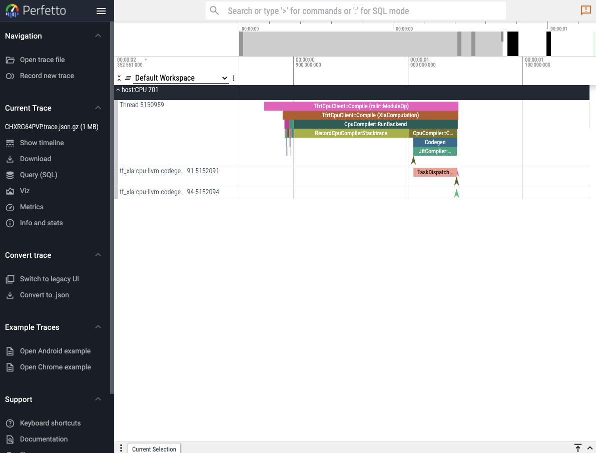
The first and easiest way to visualize a captured trace is to use the online perfetto.dev tool. Reactant.with_profiler has a keyword parameter called create_perfetto_link which will create a usable perfetto URL for the generated trace. The function will block execution until the URL has been clicked and the trace is visualized. The URL only works once.
Reactant.with_profiler("./"; create_perfetto_link=true) do
    mylinear = Reactant.@compile linear(x, W, b)
    mylinear(x, W, b)
end
Note
It is recommended to use the Chrome browser to open the perfetto URL.
XProf
XProf is a complete web UI to analyze the log files captured by Reactant. It can be installed in the following manner:
pip install xprof # or xprof-nightlyLaunching xprof is then as simple as:
xprof --logdir=./which will then make the xprof interface available on port :8791 by default.
Tensorboard
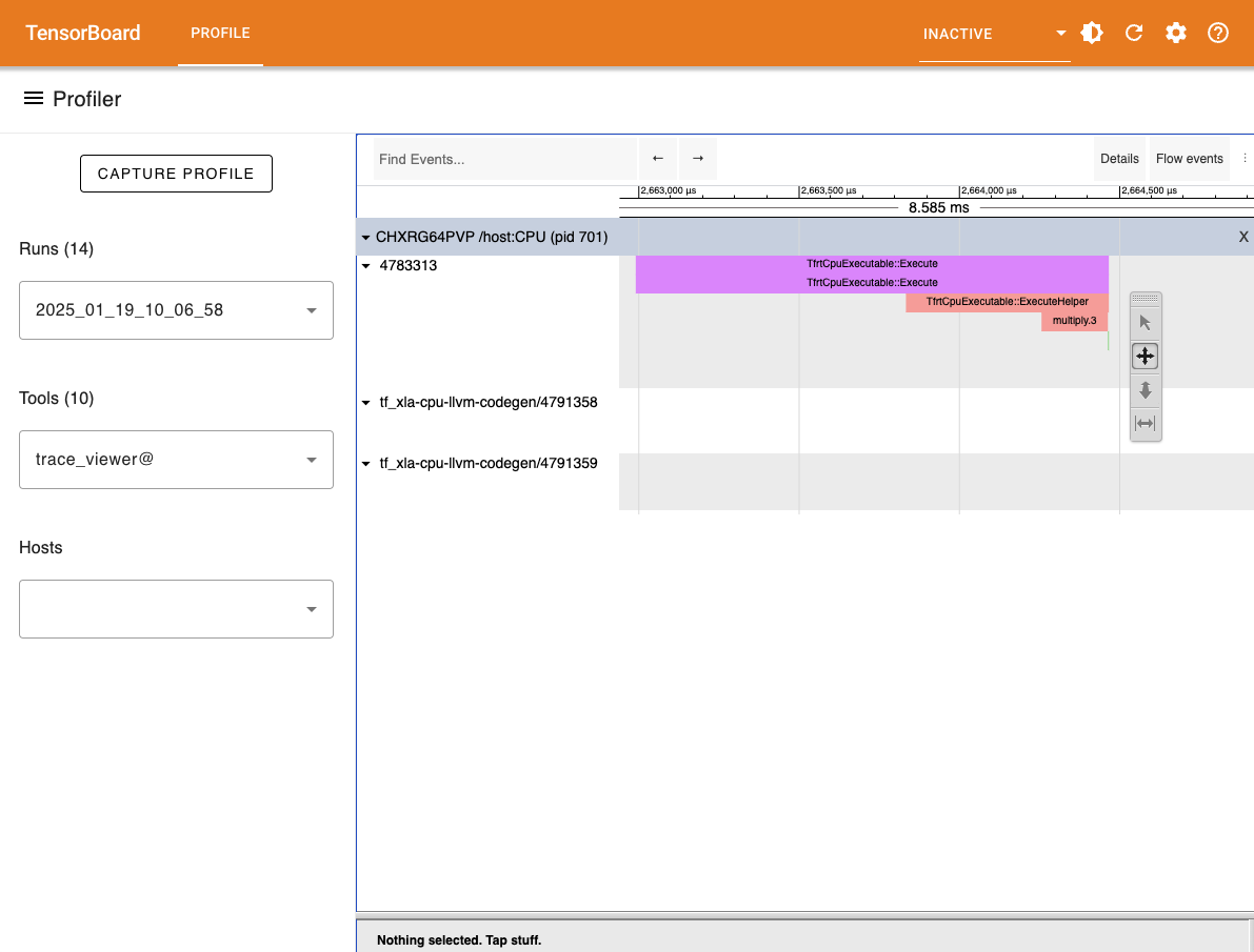
Another option to visualize the generated trace files is to use the tensorboard profiler plugin. The tensorboard viewer can offer more details than the timeline view such as visualization for compute graphs.
First install tensorboard and its profiler plugin:
pip install tensorboard tensorboard-plugin-profileAnd then run the following in the folder where the plugins folder was generated:
tensorboard --logdir ./Adding Custom Annotations
By default, the traces contain only information captured from within XLA. The Reactant.Profiler.annotate function can be used to annotate traces for Julia code evaluated during tracing.
Reactant.Profiler.annotate("my_annotation") do
    # Do things...
end
The added annotations will be captured in the traces and can be seen in the different viewers along with the default XLA annotations. When the profiler is not activated, then the custom annotations have no effect and can therefore always be activated.